
Albert Tseng*, Jerry Chee*, Qingyao Sun, Volodymyr Kuleshov, and Chris De Sa
Large language models (LLMs) exhibit amazing performance on a wide variety of tasks such as text modeling and code generation. However, they are also very large. For example Llama 2 70B has 70 billion parameters that require 140GB of memory to store in half precision. This presents many challenges, such as needing multiple GPUs just to serve a single LLM. To address these issues, researchers have developed compression methods that reduce the size of models without destroying performance.
One class of methods, post-training quantization, compresses trained model weights into lower precision formats to reduce memory requirements. For example, quantizing a model from 16 bit to 2 bit precision would reduce the size of the model by 8x, meaning that even Llama 2 70B would fit on a single 24GB GPU. In this work, we introduce QuIP#, which combines lattice codebooks with incoherence processing to create state-of-the-art 2 bit quantized models. These two methods allow QuIP# to significantly close the gap between 2 bit quantized LLMs and unquantized 16 bit models.
| Method | Precision | Wiki \(\downarrow\) | C4 \(\downarrow\) | ArcE \(\uparrow\) | PiQA \(\uparrow\) |
|---|---|---|---|---|---|
| Native | 16 bit | 3.120 | 5.533 | 0.597 | 0.809 |
| OPTQ | 3 bit | 4.577 | 6.838 | 0.544 | 0.786 |
| OPTQ | 2 bit | 109.820 | 62.692 | 0.253 | 0.505 |
| QuIP | 2 bit | 5.574 | 8.268 | 0.544 | 0.751 |
| QuIP# | 2 bit | 4.159 | 6.529 | 0.595 | 0.786 |
| ☞ | Our method, QuIP#, creates 2 bit LLMs that achieve near-native performance, a previously unseen result. We provide a full suite of 2 bit Llama 1 and 2 models quantized using QuIP#, as well as a full codebase that allows users to quantize and deploy their own models. We also provide CUDA kernels that accelerate inference for QuIP# models. Our code is available here. |
QuIP# relies on two main components: incoherence processing and lattice codebooks. Incoherence processing in the context of model quantization was introduced in QuIP. While QuIP used a Kronecker product to perform incoherence processing, we introduce a Hadamard transform-based incoherence approach that is more amenable to fast GPU acceleration.
Incoherence-processed weights are approximately Gaussian-distributed, which means that they are suitable for quantizing with symmetric and “round” codebooks. We introduce a new lattice codebook based on the \(E_8\) lattice, which achieves the optimal 8 dimension unit ball packing density. Our codebooks are specifically designed to be hardware-friendly by exploiting symmetries in these lattices.
In QuIP#, we follow existing state-of-the-art post training quantization methods and round weights to minimize the per-layer “adaptive rounding” proxy objective
\[ \ell(\hat W) = E_x \left[ \| (\hat W - W)x \|^2 \right] = \operatorname{tr}\left( (\hat W - W) H (\hat W - W)^T \right). \]
Here, \(W \in \mathbb{R}^{m \times n}\) is the original weight matrix in a given layer, \(\hat W = \mathbb{R}^{m \times n}\) are the quantized weights, \(x \in \mathbb{R}^n\) is an input vector drawn uniformly at random from a calibration set, and \(H\) is the second moment matrix of these vectors, interpreted as a proxy Hessian. This intra-layer formulation makes quantization tracatable for large language models. The original QuIP paper forumlated a class of adaptive rounding methods that used linear feedback to minimize \(\ell\). Within this class, the LDLQ rounding algorithm was shown to be optimal; we use LDLQ in QuIP# as well.
The main insight of QuIP is that incoherent weight and hessian matrices result in improved quantization performance. Informally, this means that weights that are even in magnitude with important rounding directions (the Hessians) that are not too large in any one coordinate are significantly easier to quantize without catastrophic error. In some sense, incoherence processing can be viewed as a form of outlier suppression across weight and activation spaces.
Definition. We say a symmetric Hessian matrix \(H \in \mathbb{R}^{n \times n}\) is \(\mu\)-incoherent if it has an eigendecomposition \(H = Q \Lambda Q^T\) such that for all \(i\) and \(j\), \(|Q_{ij}| = |e_i^T Q e_j| \leq \mu / \sqrt{n}\). By extension, we say a weight matrix \(W \in \mathbb{R}^{m \times n}\) is \(\mu\)-incoherent if for all \(i\) and \(j\), \(|W_{ij}| = |e_i^T W e_j| \leq \mu \|W\|_F / \sqrt{mn}\).
Incoherence is an important property for quantizing models. In QuIP, the incoherence condition on \(H\) is required to show that LDLQ achieves a superior proxy loss to nearest and stochastic rounding through a spectral bound on \(H\). Therefore, it is important to be able to incoherence-process weight and hessian matrices efficiently so that incoherence-processed models can be tractably deployed.
One way to do this is by conjugating \(W\) and \(H\) by random orthogonal matrices. Let \(U \in \mathbb{R}^{m \times m}\), and \(V \in \mathbb{R}^{n \times n}\) be two random orthogonal matrices. If we assign \(\tilde H \gets V H V^T\) and \(\tilde W \gets U W V^T\), \(\tilde H\) and \(\tilde W\) become incoherence processed with high probability (see QuIP for proof). One can verify that this transformation preserves the proxy objective as \[\operatorname{tr}(\tilde W \tilde H \tilde W^T) = \operatorname{tr}((U W V^T) (V H V^T) (V W^T U^T)) = \operatorname{tr}(WHW^T).\]
To construct \(U\) and \(V\) from above, we use the RHT, which is amenable to fast GPU implementation. In fact, one of the CUDA sample kernels is the RHT. The RHT performs the multiplication \(x \in \mathbb{R}^n \to \mathbb{H}Sx\), where \(\mathbb{H}\) is a \(n \times n\) Hadamard matrix (scaled by a normalization factor) and \(S\) is a \(n\) dimensional random sign vector. The RHT concentrates the entries of \(x\) and thus results in incoherent matrices through an application of the Azuma-Hoeffding inequality. Note that the Hadamard transform can be computed more efficiently than a matrix multiplication via the fast Walsh-Hadamard transform, which we employ directly for powers of 2. To handle non power-of-two values of \(n\), we perform the following algorithm:
The only consequence of performing RHT is needing to store two sign vectors per layer: \(S_U\) and \(S_V\). Since large language models have large weight and Hessian matrices, this only increases the number of bits per weight in practice by less than 0.01, or a negligible amount.
Incoherence processed weights are approximately Gaussian-distributed, meaning that they are symmetric and “round.” To take advantage of this “roundness,” we can use \(n\) dimensional codebooks that quantize \(n\) weights at once. Specifically, to quantize \(x \in \mathbb{R}^n\) to a \(n\) dimensional codebook \(C \in \mathbb{R}^{m \times n}\), we round \(x\) to its nearest distance-wise entry in \(C\). This requires \(\log_2m\) bits to represent which index in \(C\) to store, and results in \(k = \frac{\log_2m}{n}\) bits per weight.
Increasing \(n\) results in a “rounder” codebook that reduces quantization error. However, note that the number of bits per weight is determined by both the number of entries in \(C\) (m) as well as the dimension of \(C\) (n). To maintain a set number of bits per weight, a linear increase in \(n\) requires an exponential increase in \(m\). For example, a naively designed 16-dimensional codebook requires \(2^{32}\) entries to achieve 2 bits per weight, but performing lookups into a size \(2^{32}\) codebook is intractable. Thus, it is important to design codebooks that both have relatively large \(n\) while being compressible so the actual lookup happens with less than \(2^{nk}\) entries.
Geometric lattices are suitable bases for such codebooks as most lattices have inherent symmetries and certain lattices achieve optimal bin packing densities. For example, our E8P codebook based on the \(E_8\) lattice has \(2^{16}\) entries but only requires looking up into a size \(2^8\) codebook due to symmetries inherent to the \(E_8\) lattice itself – more on this later. In QuIP#, we present the E8P codebook based on the 8-dimensional \(E_8\) lattice. This lattice achieves the 8 dimensional kissing number, or the maximum number of unit balls touching a central unit ball in 8 dimensions. Interestingly, Maryna Viazovska recently won the Fields Medal in 2022 “for the proof that the \(E_8\) lattice provides the densest packing of identical spheres in 8 dimensions.”
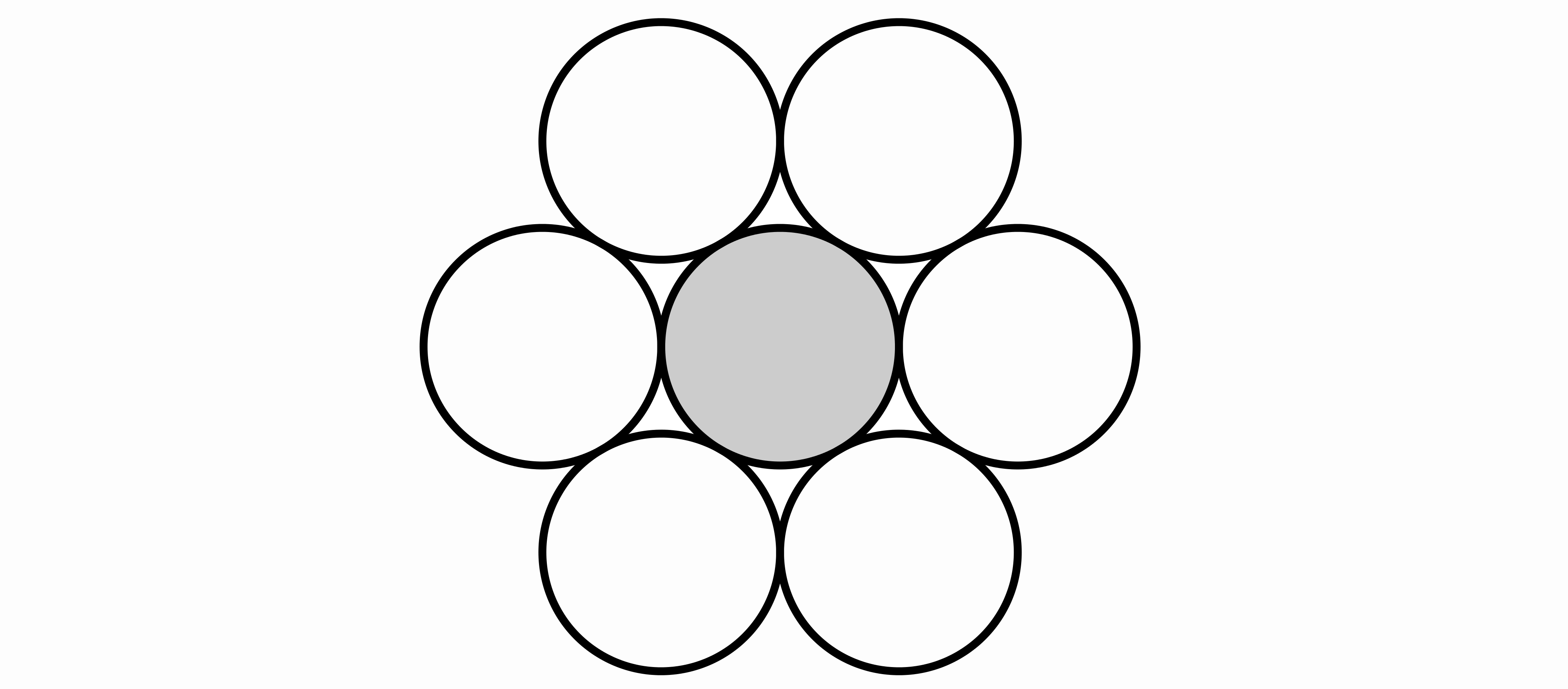
Our E8P codebook is a version of the \(E_8\) lattice intersected with a ball, padded (hence the P in E8P) to reach \(2^{16}\) entries. This results in \(k = 16/8 = 2\) bits per weight. The \(E_8\) lattice is composed of 8 dimensional all-integer or all-half integer vectors whose sum is an even number. In set-builder notation, \[E_8 = \left\{x \mid x \in \left(\mathbb{Z}^8 \cup \left(\mathbb{Z}+\frac{1}{2}\right)^8\right) \land \sum_i x_i \equiv 0 \pmod 2\right\}.\] Note that \(E_8 + \frac{1}{4}\) has the same packing density of \(E_8\) and is equivalent to \(D_8 + \frac{1}{2} \pm \frac{1}{4}\), where \(D_8\) is the set of 8 dimensional all-integer vectors with even sum. Denote \(D_8 + \frac{1}{2}\) as \(\hat{D_8}\); all elements in \(\hat{D_8}\) also have even sum parity.
Now, note that if we flip an even number of signs of an element in \(\hat{D_8}\), we get another element in \(\hat{D_8}\), whereas flipping an odd number of signs results in something not in \(\hat{D_8}\). This is due to \(\hat{D_8}\) being a half integer grid; flipping a single half integer results in changing the sum parity. Since \(\hat{D_8}\) has 8 dimensions, there are \(2^8/2 = 128\) possible “even sign flip” patterns to stay within \(\hat{D_8}\). Conversely, there are also 128 “odd sign flip” patterns.
If we start from some “source codebook” \(S\) that is a subset of \(|\hat{D_8}|\), where \(|\cdot|\) denotes the elementwise absolute value, we can use 128 odd or even sign flips to generate a subset of \(\hat{D_8}\). Each entry in \(S\) is either an odd or even number of flips away from an entry in \(\hat{D_8}\), but not both. Thus, given an entry \(s \in S\) and 7 out of the 8 sign flips, we can infer the last one from the parity of the 7 sign flips and \(s\). This lets us use the following bit pattern to store a 16-bit codeword in \(E_8 + \frac{1}{4}\): 8 bits for the entry index in \(S\), 7 bits for the sign flips of the right 7 dimensions of the entry in \(S\), and 1 bit to add or subtract \(\frac{1}{4}\).
For example, if we had the codeword 0001010110010111,
the first 8 bits 00010101 = 21 would indicate that we start
with the 21st entry in \(S\). In this
example, let this be the vector
\[\left\{\frac{1}{2}, \frac{1}{2}, \frac{1}{2}, \frac{3}{2}, \frac{1}{2}, \frac{1}{2}, \frac{1}{2}, \frac{1}{2}\right\},\]
which is not in \(\hat{D_8}\). Thus,
\(s\) requires an odd number of sign
flips to get into \(\hat{D_8}\). Then,
the next 7 bits 1001011 would indicate that we need to
negate the 1st, 2nd, 4th, and 7th from right bits. Since we need an odd
number of sign flips, the 8th from right bit is also a sign flip. The
sign-decoded vector is then
\[\left\{-\frac{1}{2}, -\frac{1}{2}, \frac{1}{2}, \frac{3}{2}, -\frac{1}{2}, \frac{1}{2}, -\frac{1}{2}, -\frac{1}{2}\right\},\]
which we can verify is in \(E_8\).
Finally, the last bit 1 indicates that we need to add \(\frac{1}{4}\), so the final decoded vector
is
\[\left\{-\frac{1}{4}, -\frac{3}{4}, \frac{3}{4}, \frac{7}{4}, -\frac{1}{4}, \frac{3}{4}, -\frac{1}{4}, -\frac{1}{4}\right\},\]
which is in \(E_8 + \frac{1}{4}\) as desired.
Putting this all together, this lets us decode a size \(2^{16}\) codebook by looking up into only a size \(2^8\) codebook (namely \(S\)) and performing some operations. On hardware, this means that we can store the smaller \(2^8\) codebook in local caches, avoiding performance killing memory accesses that the larger \(2^{16}\) codebook would require. The question remains then of how to choose \(S\). In our implementation, we set \(S\) to be the 227 elements of \(|\hat{D_8}|\) with norm \(\le \sqrt{10}\) plus 29 elements from \(|\hat{D_8}|\) that have norm \(\sqrt{12}\). The exact elements chosen can be found in our code.
The \(E_8\) lattice works well for low bitrates, but quickly becomes intractable at higher bitrates. For example, a 4 bit \(E_8\)-based codebook would have size \(2^{4*8} = 2^{32}\). Projecting onto a size \(2^{32}\) codebook is intractable, and even using a “smarter” packing like E8P would still require projecting onto \(2^{24}\) elements. To deal with this issue, we use residual vector quantization (RVQ) to get the benefits of lattice codebooks and QuIP# at higher bitrates. RVQ quantizes a vector \(x\) to \(p\) bits with a set \(q\) of \(q_i\) bit codebooks (denoted \(RVQ(x, p, q)\) where \(p = \sum_{0 \le i < |q|} q_i\)) by repeatedly quantizing the quantization residual. That is, \(RVQ(x, p, q) = \sum_{0 \le i < |q|} \delta_i\) where \(\delta_i = Q_{q_i}\left(\frac{x - \sum_{0 \le j < i}\delta_j}{s_i} \right) s_i\), \(Q_{q_i}(\cdot)\) denotes quantizing to a \(q_i\) bit codebook, and \(s_i \in \mathbb{R}\). Using RVQ, we can quantize to 4 bits by quantizing with the 2 bit E8P codebook twice. We can also quantize to 3 bits by using the 2 bit E8P codebook and a 1 bit \(E_8\) codebook (elements of \(E_8\) with norm \(\le 2\) and 15 elements of \(E_8\) with norm 4). We present results for these 3 and 4 bit models under “E8P RVQ.”
To show the optimality of our lattice codebooks, we plotted the minimum achievable elementwise MSE of quantizing a \(n\)-dimensional multivariate Gaussian to various \(k\) bit codebooks. To create each codebook, we intersected a ball with the base lattice and increased the radius of the ball to get more bits. The half integer codebooks are formed from the \(n\)-dimensional half integer grids.
Specifically, each point in the graph below plots \((k, y)\) where
\[y = \min_{s \in \mathbb{R}^+} \frac{1}{n}\left\|\mbox{quantize}\left(\frac{\mathcal{N}(0_n, I_n)}{s}, \mbox{codebook}\right)s - \mathcal{N}(0_n, I_n)\right\|^2\]

The \(E_8\)-based codebooks achieves lower MSEs than all other codebooks, including those based on the \(D_4\) lattice that achieves the 4 dimensional kissing number. This figure also shows the importance of having a large number of columns \(n\). Increasing the number of columns decreases the error for the half integer grid, as the resulting codebook is more “round.” Since the E8P codebook is actually the union of two shifted codebooks, each of which is a ball intersected with \(\hat{D_8}\), it is not perfectly round. This is reflected in the MSE plot, where it sits slightly above the \(E_8\) line. However, there does not exist a \(E_8\) codebook with exactly 2 bits, so E8P is still practically superior.
Here, we present an overview of quantization results using QuIP# on Llama 1 and 2 models. Full results are available here.
All models were quantized using the Hadamard transform for incoherence processing and a weight scale factor of roughly 0.9 times the optimal scale for a multivariate Gaussian to compensate for inter-layer interactions. Furthermore, all Llama 2 models were evaluated using a context lenth of 4096 and all Llama 1 models were evaluated with context length 2048; these numbers match the context length the models were trained with. These and other models can be found in our Hugging Face repository.
The table below contains results for all Llama 1 and 2 models when quantized to 2 bits using the E8P codebook. QuIP# achieves excellent performance across all model sizes on both language modeling and zero shot tasks. Furthermore, on the zero-shot tasks (ArcC, ArcE, BoolQ, PiQA, WinoGrande), QuIP# models achieve near-native performance with minimal degradation.
| Model | Method | C4 | Wiki | ArcC | ArcE | BoolQ | PiQA | WinoGrande |
|---|---|---|---|---|---|---|---|---|
| 2-70B | fp16 | 5.533 | 3.120 | 0.480 | 0.597 | 0.766 | 0.809 | 0.768 |
| 2-70B | QuIP# 2 bit | 6.529 | 4.158 | 0.472 | 0.595 | 0.791 | 0.786 | 0.742 |
| 2-13B | fp16 | 6.520 | 4.574 | 0.443 | 0.580 | 0.690 | 0.790 | 0.699 |
| 2-13B | QuIP# 2 bit | 8.755 | 6.058 | 0.371 | 0.501 | 0.665 | 0.757 | 0.636 |
| 2-7B | fp16 | 7.036 | 5.116 | 0.406 | 0.535 | 0.710 | 0.769 | 0.670 |
| 2-7B | QuIP# 2 bit | 12.062 | 8.224 | 0.325 | 0.428 | 0.623 | 0.712 | 0.624 |
| 1-65b | fp16 | 5.811 | 3.532 | 0.463 | 0.588 | 0.823 | 0.809 | 0.771 |
| 1-65b | QuIP# 2 bit | 6.744 | 4.566 | 0.436 | 0.569 | 0.817 | 0.805 | 0.736 |
| 1-30B | fp16 | 6.130 | 4.101 | 0.453 | 0.590 | 0.684 | 0.801 | 0.728 |
| 1-30B | QuIP# 2 bit | 7.471 | 5.317 | 0.429 | 0.545 | 0.669 | 0.779 | 0.718 |
| 1-13B | fp16 | 6.798 | 5.091 | 0.444 | 0.599 | 0.684 | 0.792 | 0.701 |
| 1-13B | QuIP# 2 bit | 8.425 | 6.381 | 0.387 | 0.536 | 0.647 | 0.750 | 0.669 |
| 1-7B | fp16 | 7.343 | 5.677 | 0.415 | 0.525 | 0.731 | 0.774 | 0.670 |
| 1-7B | QuIP# 2 bit | 10.970 | 8.286 | 0.352 | 0.464 | 0.647 | 0.720 | 0.624 |
Using residual vector quantization (RVQ) allows us to get the benefits of vector quantization and lattice codebooks at higher bitrates. The charts below plot the perplexity gap of QuIP#, AWQ, and OmniQuant models at 3 and 4 bits to a FP16 baseline. We report numbers without grouping (W3A16) since grouping adds bits. For example, a groupsize of 128 adds \(\frac{16}{128} = \frac{1}{8}\) bit per weight, which is a significant difference. AWQ and OmniQuant numbers are from the OmniQuant paper. At both bit levels, QuIP# significantly closes the gap to FP16, outperforming AWQ and OmniQuant. QuIP# 3 bit approaches AWQ 4 bit and in some cases even outperforms AWQ 4 bit.
